The easiest way for configuring the parameter setting of an EA when working
with the JCell framework is to define all the desired parameterization into
a simple configuration file. This option, provided by the ReadConf
class, has clear advantages, since the user does not need to know the inner
details of JCell codification, like the variable names and their data type.
Additionally, we can easily change both the parameter settings of our EA and
the algorithm itself without the need of compiling the code. These features
make our framework accessible to those researchers belonging to any field, since
it is not needed to have any knowledge in programming languages for using JCell.
The only thing they have to do is to edit the configuration file for
setting the parameterization and then run the JCell.class file.
An example is the following command line:
java JCell config.conf
Therefore, using this kind of configuration file, the functionality and the
easy of use of JCell is highly strengthened. And this is a really important
issue for its success and acceptance by the scientific community. The configuration
file is composed of pairs:
In the figure below we can see two example configuration
files for JCell. The one on the left is a typical configuration for a cGA (Algorithm
= cellular), in which the visiting order of individuals in the
breeding loop is defined by an asynchronous Fixed Random Sweep policy (UpdatePolicy
= Asynchronous FRS), and the population shape is set to 20x20
(Population = (20,
20)). The evolution of the individuals in the population is
displayed (ShowDisplay
= true), being updated every generation, and JCell will print
on the
standard output some significative information of the evolution of the population
during the run (Verbose
= true). The problem we want to solve is the combinatorial optimization
ECC
problem (Problem
= problems.Combinatorial.ECC), whose class is implemented in
the package problems.Combinatorial
of JCell. The termination condition of the algorithm is to find the optimal
solution to the problem (which is given in the class implementing the problem),
or to reach a maximum of 1 million fitness function evaluations (EvaluationsLimit
= 1000000). The chromosome of individuals must be composed by
binary genes for solving combinatorial optimization (Individual
=
jcell.BinaryIndividual), and the neighborhood structure we want
to use is Linear5 (Neighborhood
= jcell.Linear5), from which the second parent will be selected
by binary tournament selection (SelectionParent2
= jcell.TournamentSelection). The other parent (which will be
selected firstly) is the current individual itself (SelectionParent1
= jcell.CenterSelection). The two selected parents are never
allowed to be the same individual in JCell. The two points recombination operator
(Crossover = operators.Dpx)
is applied to these to parents with probability 100\% (CrossoverProb
= 1.0), and the newly generated offspring is always mutated
(MutationProb = 1.0)
using the binary mutation operator (Mutation
= operators.BinaryMutation). The genes of the chromosome are
mutated with probability 1/L,
being L the length of the chromosome. Finally, the offspring replaces the current
individual in the population only if it has a better (or equal) fitness value
(Replacement = jcell.ReplaceIfNonWorse).
In the right side of the figure we can see how easy is
to run a steady-state multi-objective GA with JCell just by changing a few key
parameters in the previously explained configuration file. Just by changing
the Algorithm
key to steady-state
we get a steady-state GA. The population in a panmictic algorithm (both steady-state
and generational) is a pool of individuals, and thus it has no structure nor
a concrete shape. Therefore, we directly set the population size in this file
instead of its shape (Population
= 400). The problem we want to tackle is the
so called Deb's
problem (Problem
= problems.MO.Deb), and the maximum number of fitness function
evaluations is set to 25000, as it is usual in multi-objective optimization.
Deb's problem requires a codification of Double
genes for representing the variables (Individual
= jcell.RealIndividual), and thus we have to use proper recombination
(simulated binary -Crossover
= operators.SBX-) and mutation (non uniform mutation -Mutation
= operators.NonUniformMutation-) operators for this kind of
chromosome representation. Finally, the neighborhood must not be specified since
the whole population will be considered the neighborhood for the steady-state
GA.
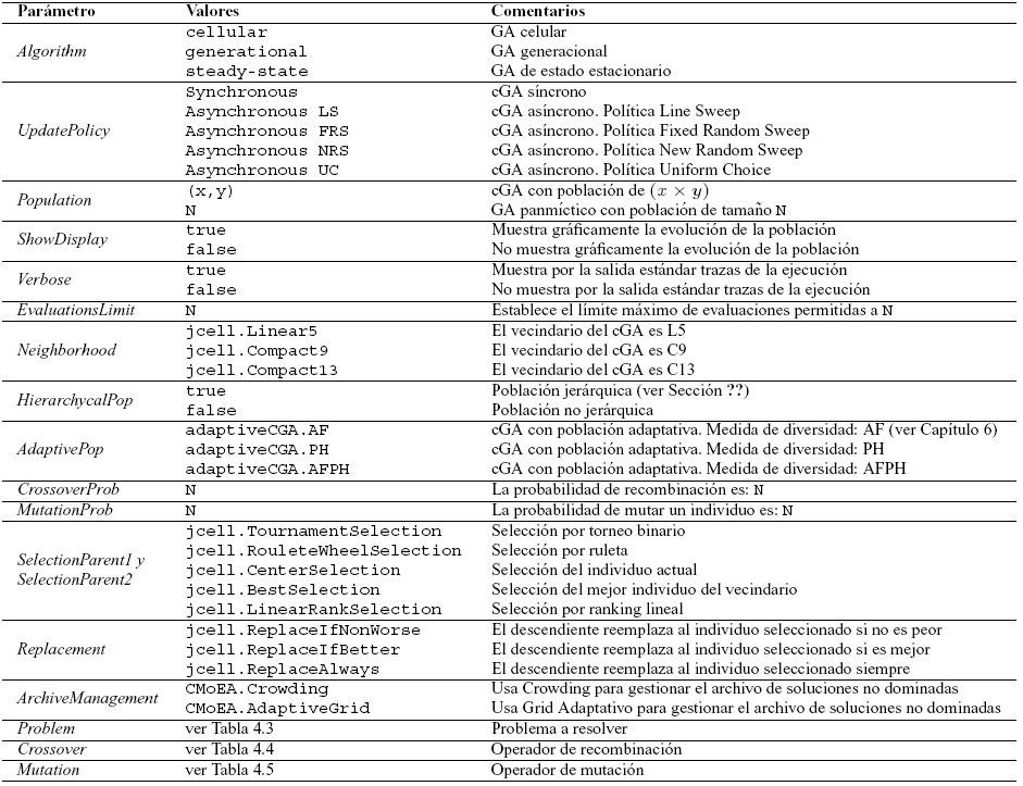
In Table 1 we show the main configuration parameters we can use with JCell,
togethter with the values they can have and a brief explanation (in Spanish
for the moment, sorry about that).
Table 1. Main JCell configuration Parameters
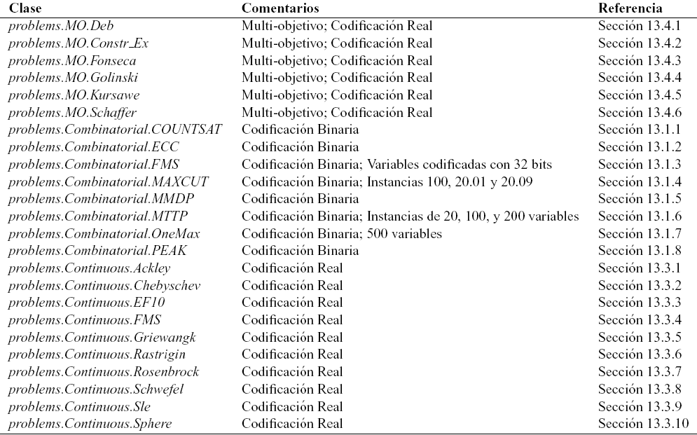
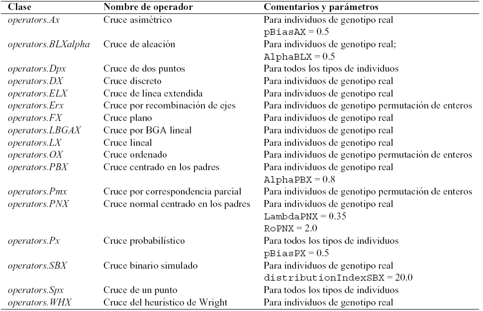
The main problems included in JCell, as well as the available recombination
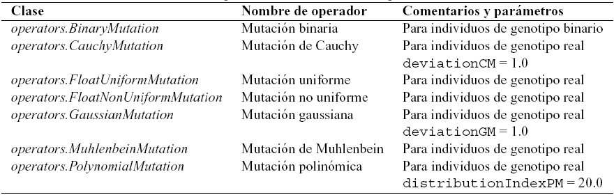
and mutation operators in JCell are shown in tables 2, 3, and 4, respectively.
Table 2. Problems available in JCell.
Table 3. Recombination operators available in JCell.